Distributions

In statistics, are often interested in describing a random variable by its distribution. That means, we assume that there exists a rule, by which the data has been randomly generated. This is true even if the data itself is not random; you can see distributions as an efficient way of describing data.

When analyzing data in practice, you are often interested in finding out which distribution describes the data best. This chapter outlines a few common distributions.

Probability mass functions

The probability mass function (pmf) defines probabilities for a discrete random variable. The pmf gives the probability for each possible outcome as a number between 0 and 1. Sometimes the pmf is an equation, but it could also be a table.

In any case, the sum of the probabilities for all possible outcomes must be equal to 1.0.

Example

You have a population of 100 Adelie penguins and 200 Gentoo penguins. If you pick a penguin at random, the probability mass function is:

\[p(species) = \frac{n_{species}}{n_{total}}\]

So you get \(p(Adelie) = 0.333\) and \(p(Gentoo) = 0.666\).

Probability density functions

If you are describing a continuous random variable, it does not make any sense to consider a single value Instead, you consider the probability that a value is within an interval. The probability density function allows you to calculate probabilities for continuous variables. The probability of a value being in an interval \([a, b]\) is the area under the curve.

\[f([a, b]) = p(a \leq X \leq b)\]

The total area under the curve from negative to positive infinity has to be 1.0.

---

Uniform Distribution

In a Uniform Distribution, all probabilities are the same. A dice roll is a good example. The Uniform Distribution applies to both discrete and continuous variables.

For the discrete case, the Uniform Distribution has the probability mass function:

\[p(x)=\frac {1}{n}\]

Example

The outcome of a single dice roll is uniformly distributed.

---

Binomial Distribution

When a random event (e.g. a single coin toss) has two possible outcomes, it follows the Bernoulli Distribution. This is an ambitious term for a very simple fact:

• one outcome occcurs with the probability \(p\)

• the other outcome occurs with the probability \(1-p\)

The situation becomes more interesting if multiple events are examined (e.g. a series of coin tosses). Such a series follows the Binomial Distribution, and is described by the probability of a single event p, the number of experiments n and the number of positive outcomes k.

The Binomial Distribution has the probability density function:

\[f(p,n,k) = {\binom {n}{k}}p^{k}(1-p)^{n-k}\]

Where the expression \({\binom {n}{k}}\) is called a binomial coefficient. You can calculate it by:

\[{\binom {n}{k}} = \frac{n!}{k! (n-k)!}\]

---

Geometric Distribution

When a Bernoulli experiment is repeated until an event occurs, you can apply the Geometric Distribution. The Geometric Distribution describes the time until success or failure (e.g. customer churn). It is a discrete version of exponential decay. The Geometric Distribution for k steps has the probability mass function:

\[f(x)=p(1-p)^{k-1}\]

The mean of the pmf is \(\frac {1}{p}\)

---

Poisson Distribution

Rare events can be described by the Poisson Distribution. A rare event is characterized by its frequency \(\lambda\), the number of occurences per time step (e.g. the number of events per hour, per minute etc.). The Poisson Distribution has the probability mass function for k events:

\[\frac {\lambda ^{k}e^{-\lambda }}{k!}\]

The Poisson Distribution also works for frequent events, but for \(\lambda \tilde> 15\) you might as well use the Normal Distribution.

---

Normal Distribution

by Ainali - Own work, CC BY-SA 3.0

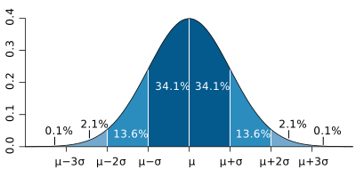
The Normal Distribution is by far the most frequently observed distribution. It is a continuous distribution with the probability density function:

\[f(x)={\frac {1}{\sigma {\sqrt {2\pi }}}}e^{-{\frac {1}{2}}\left({\frac {x-\mu }{\sigma }}\right)^{2}}\]

with the mean \(\mu\) and the standard deviation \(\sigma\) . A normal distribution with \(\mu=0\) and \(\sigma=1\) it is called the Standard Normal Distribution.

One pleasant property of the Normal Distribution is that it defines a clear interpretation of the standard deviation:

• 68.2% of the values are within one standard deviation from the mean

• 95.4% of the values are within two standard deviations from the mean

• 99.7% of the values are within three standard deviations from the mean

Hint

In a Google spreadsheet you can use the function NORM to calculate the probability that the value of a normally distributed variable is below the given threshold.

E.g. to calculate the probability that a penguin has a beak length of 45 mm or below when the beak lengths are normally distributed with a mean of 40 mm and a standard deviation of 2.5 mm, use the formula:

=NORM.DIST(45.0, 40.0, 2.5, TRUE)

The probability that the beak is longer than 45 mm is 1 minus the resulting value.

---

The Central Limit Theorem

The Central Limit Theorem states that a sum of many distributions approximates the Normal Distribution. For instance you get a Normal Distribution from:

• the sum of multiple dice rolls for many dice

• the number of heads for many dice rolls

• the sum of multiple runs of a Geometric Distribution

• the Poisson Distribution for a high value of k

The Central Limit Theorem even applies if the added distributions are different, as long as there is not a single dominant one. This is the mathematical explanation why we observe so many Normal Distributions in nature.

See also

• More detailed description of the concepts in this chapter