Gradient Descent
Gradient Descent is the most important algorithm in Machine Learning.
Warmup Puzzle
Identify the seven concepts in the diagram using the syllables:
AL BAL CE CON DI DI ENT ER FUNC
GING GING GLO GRA LOC LOSS MET
MI MI MUM MUM NI NI ON PARA
SPA TI VER VER

Key Concepts
concept |
description |
|---|---|
Gradient Descent |
iterative algorithm to find optimal parameters |
Gradient |
partial differential over all features |
Loss function |
the function that is optimized |
Learning rate |
factor that determines the size of steps |
Stochastic Gradient Descent |
variant using randomly selected points |
Mini-Batch Gradient Descent |
variant using random samples of points |
Background
Gradient Descent is an algorithm used to fit the parameters of a model. More technically, Gradient Descent finds the minimum of a loss function in a parameter space.
Loss function means the metric used to measure the quality of a model. It is not the estimate \(\hat y\) of the dependent variable.
Parameter space means that we consider all possible combinations of parameters. Because a model might have many parameters, this space is multi-dimensional. Of course, it is too complex to try out all possible combinations.
Instead, we move through the parameter space in iterative steps, minimizing the loss function. The key equation for calculating the weight modification \(\triangle a\) is:
This equation calculates the gradient of the loss function. The variable \(\eta\) is called the learning rate. The learning rate is multiplied with the gradient of the loss function.
What is a gradient?
The gradient is the slope of a function in each considered dimension. In our case, it is the first derivative of the loss function.
Unfortunately, we cannot use a simple derivative function, because we have to differentiate by multiple parameters. This is called a partial differential or Jacobian.
Therefore, the resulting gradient of the loss function \(loss(a)\) is a vector containing all its partial derivatives at the point a
What is a loss function?
The minimized function is called the loss function. It depends on the optimization problem, typically:
MSE in linear regression
log-loss in binary classification
crossentropy in multinomial classification
hinge loss in SVMs.
Many applications use their own, custom loss functions.
Pseudocode
The Gradient Descent Algorithm starts with a random guess and performs minimization steps until it reaches optimal values for the parameters.
Here is the pseudocode:
1. set all model parameters to random values
2. calculate the partial derivative
   of the loss function for each parameter
3. multiply each derivatives with the learning rate
4. modify the model parameters by the resulting vector
5. repeat steps 2-4 until the loss function does not change
Stochastic Gradient Descent
When you have lots of data, the standard GD algorithm using all data points at every step becomes slow. There are two similar solutions:
Stochastic Gradient Descent (SGD) uses one randomly chosen data point at a time.
Batch Gradient Descent uses randomly chosen subsets. This is the default when training neural networks.
Exercise: Gradient Descent from Scratch
Step 1: Load the data
Add the missing imports to load the file part1/linear07.csv
and add a dummy column:
df = pd.read_csv("linear07.csv")
df["bias"] = 1
Inspect the data to make sure you have the right number of rows/columns.
Then extract the dependent and independent columns
X = df[[...]]
ytrue = df[...]
Step 2: The Model
In a nutshell, our gradient descent algorithm will optimize the parameters of a linear function in such a way that the error between the output of that function (\(\hat y\)) and the actual values (y) becomes minimal.
We assume a linear function to approximate our data set:
Here, \(a_0\) is the intercept, and the other \(a_i\) are the slopes.
To start, write a Python function called linear_model() that
accepts two arguments: the data and the parameters
and returns a list of “predicted” y values based on those parameters.
# insert: X, a, dot, return
def linear_model(X, a):
    ___ np.___(___, ___)
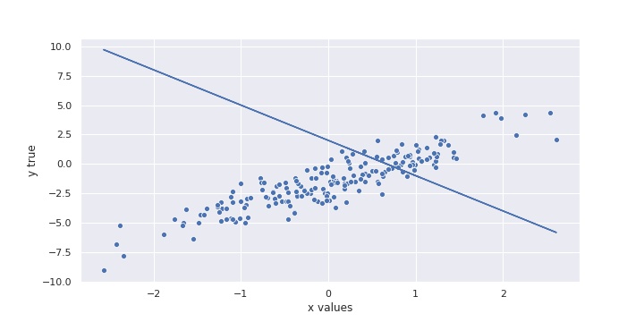
To check if your function works, try inputting random values into your function and plot the results – even if it’s an intentionally bad “guess”!
plt.plot(df["x1"], linear_model(X, -3.0, 2.0))
Step 3: The Loss Function
Our code is working, but of course the parameters we gave were bad! But that’s okay – we have to start from somewhere! And it shouldn’t matter too much how bad our initial prediction was, because it’s going to be the algorithm’s job to find the best parameters.
We (as humans) can visually tell from the plot that our initial parameters gave us a bad prediction / line of best fit.
But how can a computer tell that it’s “bad”?
We need a way of quantifying the error (or loss) between the predicted and actual values. In Machine Learning, this is referred to as a loss function. Here we will use the Mean Squared Error as a loss function:
Write a python function called mse that encodes the equation above –
accepting X, ytrue and the parameters a as arguments – and returns a single value
for the mean-squared-error.
# insert into the code: mse, mean, ytrue, yhat
def ___(ytrue, yhat):
    return np.___((___ - ___) ** 2)
If you wrote your function correctly, then the following assert statement should not return an error.
a = np.array([1.0, 1.2, 1.4, 1.6])
b = np.array([0.2, 0.4, 0.6, 0.8])

assert round(mse(a, b), 2) == 0.64
Step 4: The Gradient
The essence of gradient descent is – after determining the error between the predicted values and the actual values – deciding by how much to tweak each of the parameters in such a way that the new values for the parameters result in a smaller loss than before! So for our vector of model parameters (a=[a0, a1]), we need to calculate…
so that for the new a the MSE should be smaller than before.
How do we calculate an appropriate change for each parameter (Δa) that achieves this objective? Well, as seen in a few of the images in the material above, the delta part of the equation evaluates to:
The toughest part about implementing the algorithm is understanding what the ∇ loss(a) part means. This term represents the gradient of the loss function for each model parameter inside a. Another way of saying this is calculating the first-order partial derivatives of the loss function with respect to each of the model parameters. And since we are dealing with more than one parameters in this example, we need to calculate a partial derivative.
Write a python function called calc_gradient that takes 3 arguments:
the X data, ytrue and the parameters a.
It should calculate the numeric partial derivative for
each parameter based on a small incremental change da,
and then return the 2 partial derivatives.
The resulting list of partial derivates is called the gradient.
Some of the code is already filled in to help you get started:
def calc_gradient(X, ytrue, a):

  epsilon = 0.0001  # a tiny increment
  ypred = ...
  mse_old = ...

  # derivative for first parameter
  a1_change = a.copy()
  a1_change[0] += epsilon
  ypred_a1 = ...
  mse_a1 = ...
  deriv_a1 = (mse_a1 - mse_old) / epsilon

  # derivative for second parameter
  ...

  return [...]  # all partial derivatives
Hint
Think of how to incorporate the linear_model function that you created before.
Hint
You don’t need to work out the analytical solution to the derivate of the loss function. You can approximate it numerically using the definition of the derivative!
Step 5: Repeat
Implement the gradient descent algorithm! For this, you’ll need to run a loop.
Start by initializing a few variables. For example:
LEARNING_RATE = 0.1  # start with a small learning rate
MAX_ITER = 100

a = np.random.random(size=...)  # random starting values
Transcribe the following pseudo-code into python:
Repeat the following steps `MAX_ITER` times.
In each iteration of the loop:

1. Calculate the gradient of the loss function
   with respect to each model parameter.
2. If the gradient becomes close to zero, exit
3. Update each model parameter using the gradient
4. Print the MSE and all variables to check if they
   are converging.
Step 6: Experiment
Make the learning rate very small and/or very large. What happens?
Step 7: Plot
Plot the loss function over time.
Recap Questions
Which function are Gradient Descent algorithms minimizing?
What is a local optimum?
How much is the gradient at the minimum?
Do all runs of the Gradient Descent algorithms lead to the same solution?
If the training loss goes up consistently, what is happening? How can you fix this?
When is Stochastic Gradient Descent a better option?
When would a Gradient Descent algorithm fail to find the optimal solution?
by Paul Wlodkowski