Descriptive Statistics¶

Encounter with Penguins¶

One morning, Lumi is alone on the bridge. He is cruising through the cold waters of the far southern sea. The submarine is gently sliding through a large school of fish. Suddenly many large projectiles are splashing into the water in front, left and right of the ship. Lumi immediately sounds the alarm:

"WE ARE UNDER ATTACK!"

Lumi gets ready for an evasive maneuver: nose-diving to the deeper depths. Only then, he realizes, that the projectiles are really some kind of animals. They dive deep into the water, then rise up and go after the fish in an underwater ballet. Lumi is amazed. Never has he seen anything like that before.

As the rest of the crew rushes to the bridge, he whispers:

"Look, we have found the penguins!"

Conduct a preliminary scan of the swimming penguins:

import seaborn as sns

df = sns.load_dataset("penguins")
df = pl.from_pandas(df)

The Goal of Descriptive Statistics¶

Once your data is tidy and you have created a few exploratory plots, you usually want to describe your data in more detail. This is where Descriptive Statistics come in. This is an obligatory step whenever you are working with data whether you want to deliver an expert opinion, train a fully automated Machine Learning algorithm or monitor data in production. Statistics go very deep sometimes, but you can safely start with a few straightforward metrics. You find an overview here.

A good step to start with is to write down questions you are interested in, e.g.:

how many penguins are there?
how large are their beaks?
are there any subgroups?
are there any exceptionally small or tall penguins?

The descriptive statistics metrics help you to come up with answers that are numbers. Let's look at a few of them.

Measures of Centrality¶

When looking at a single variable (a column in your tidy data), the first thing you want to know is where the data is located. The three metrics to start with are:

The arithmetic mean¶

The arithmetic mean is the sum of all data points divided by their number:

\[\bar x = \frac{1}{n} \sum_i (x_i)\]

It can be calculated in a single line:

df["bill_length_mm"].mean()

Note

polars by default puts out numbers with maximum precision. In a report this can be very misleading and suggest your calculations are more precise than they actually are. Use round() or f"{number:6.2f}" to round the numbers. One or two decimal places are usually enough.

The median¶

The median sorts the data points and then takes the point in the middle (or the average of two if the number is even).

df["bill_length_mm"].median()

The median is less prone to outliers than the mean.

Try adding a godzilla-sized penguin to the list and see how both metrics change: In polars, there is no direct way to change a value in a column, but you can use the when-then-otherwise construct. But before that, you need to convert the pandas dataframe to a polars dataframe:

df = df.with_columns(
   pl.when(pl.arange(0, pl.len()) == 1)
   .then(2000)
   .otherwise(pl.col("bill_length_mm"))
   .alias("bill_length_mm")

)

The mode¶

The mode is simply the most frequent value of a variable. It makes more sense if your variable is an integer, ordinal or category value, and less with float scalars.

df["species"].mode()

In a scalar variable, you would also want to check if there are multiple modes. A good tool for checking modes is the histogram:

df["bill_length_mm"].hist(bins=20)

Measures of Dispersion¶

The second aspect of a single variable is how much it is spread around the center. Again, you have several options that are complimentary:

The range¶

The range is simply the word used by statisticians for the distance between the minimum and maximum value.

range = df["bill_length_mm"].max() - df["bill_length_mm"].min()

The standard deviation¶

A metric less prone to outliers is the standard deviation, or the square root of squared distances from the mean:

\[sd = \sqrt{\frac{1}{n} \sum_i (x_i - \bar x)^2}\]

An intuitive description of the standard deviation is that roughly 68% of the values are within one standard deviation from the mean, assuming a normal distribution (sorry it does not get more intuitive than that).

df["bill_length_mm"].std()

The standard deviation is also the square root of the variance (which is used less frequently).

Quartiles and everything¶

Quartiles are the ranges in which portions of 25% of the data are found. You can calculate these and lots of other statistics with a one-stop function:

df["bill_length_mm"].describe()

Distributions¶

A key question in the first two parts is: Does my data consist a homogeneous group or does it really consist of two major sub-groups. Without going into the details of testing statistical hypotheses (which is very difficult to do right) you may want to start with examining the histogram of a variable. What you want to check is:

is there more than one group (monomodal, bimodal or multimodal distribution)?
is there a predominant distribution?

You should be able to distinguish the following distributions visually: uniform, normal, standard normal and power-law (long tail) distribution.

Correlation¶

When you want to describe more than one variable, things obviously get more complicated. Here are two things to start with:

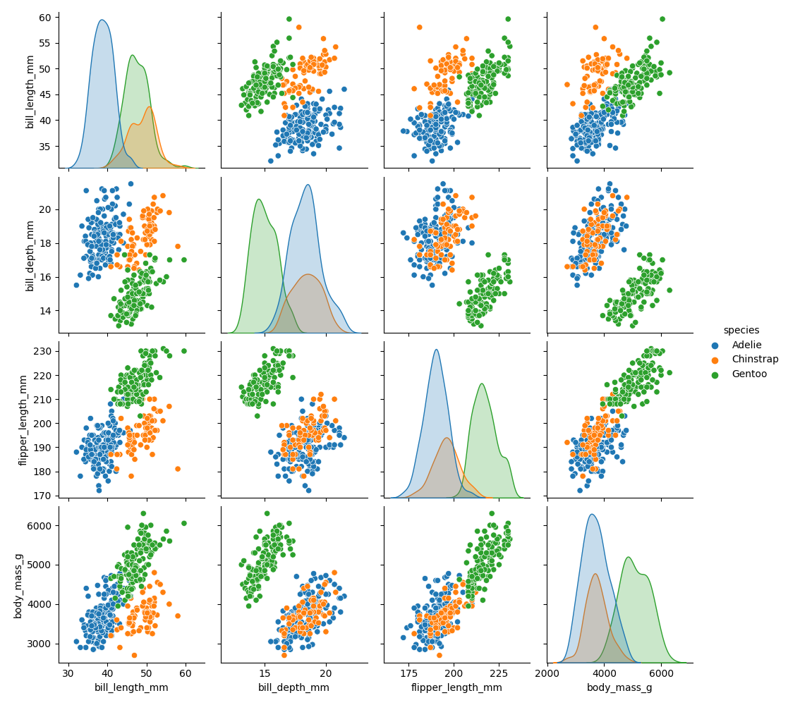
Inspect a scatter plot¶

In a scatter plot, you want to check if there are any visible sub-groups, linear or other correlations or if the data is simply a cloud of dots:

sns.scatterplot(data=df, x="bill_length_mm", y="bill_depth_mm", hue="species")

To go for a full swing, try the pairplot:

sns.pairplot(df, hue='species')

Correlation coefficients¶

A correlation coefficient describes what proportion of one variable can be explained by the other using a linear model. The correlation coefficients mean roughly:

value	meaning
1.0	perfect positive correlation
0.0	completely random
-1.0	perfect negative correlation

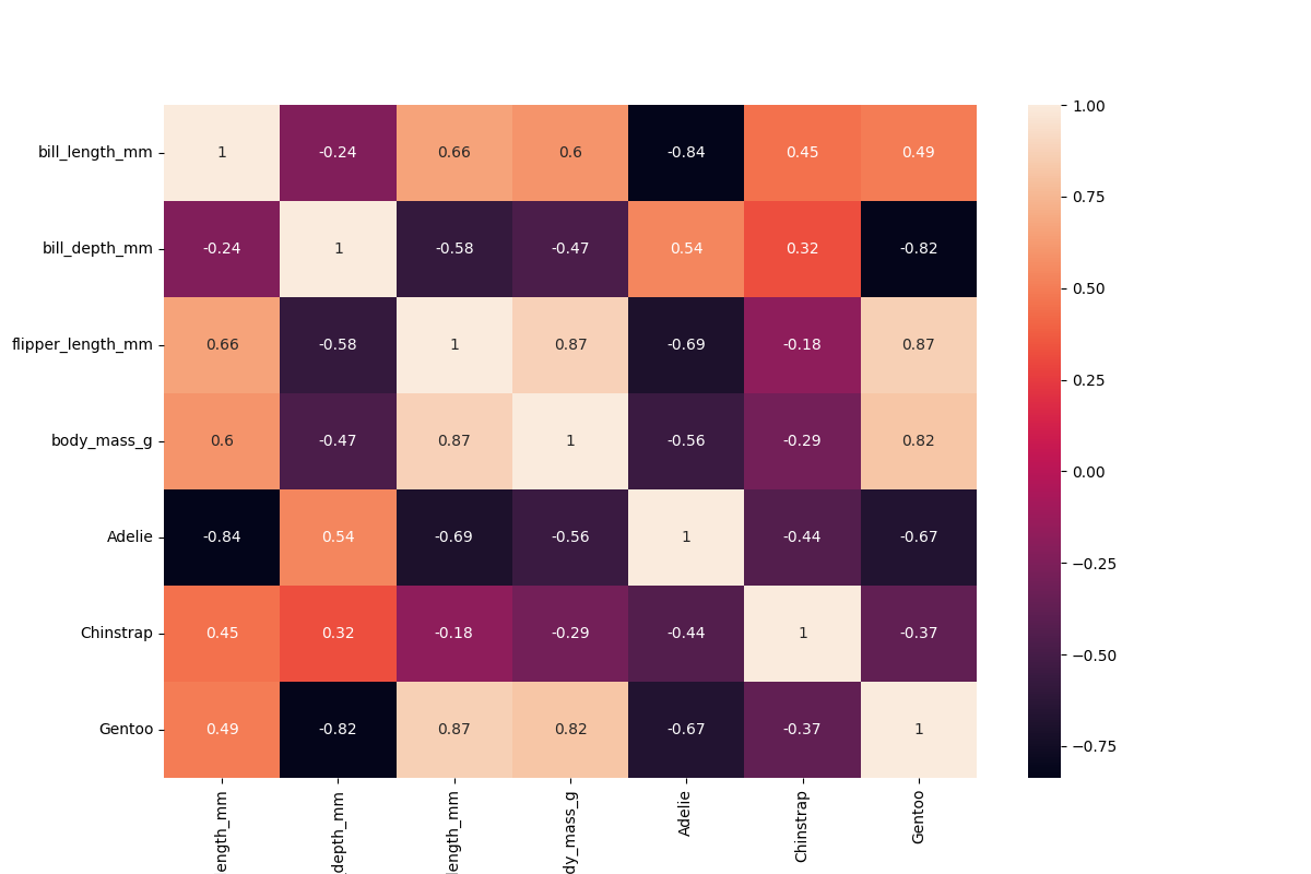
Calculating correlation coefficients for all scalar columns in pandas is easy enough:

df.corr()

If you want to correlate the categorical data as well, you need to use One-Hot Encoding:

species_dummies = df.to_dummies(columns=["species"])
df_concat = df.hstack(species_dummies)

Warning

Correlations can be very easily misleading. See next section.

The correlations can be plotted very nicely if you make some extra space for the labels:

plt.figure(figsize=(12,8))
sns.heatmap(df.corr(), annot=True, vmin=-1.0, vmax=1.0)

Confounding Factors¶

If the data has significant subgroups, the correlation coefficients might not give you the full picture. The underlying groups might be more important than the actual correlation. In that case, the groups are called a confounding factor. Confounding factors can blur the information in a correlation coefficient or even turn it around!

Identifying confounding factors is not easy and often not visible from the data alone. This is why domain expertise is indispensible!

Challenge¶

Examine the data of the penguins. Answer the following questions:

calculate the total weight of all penguins
calculate the mean flipper length over all penguins
calculate the median flipper length over all penguins
calculate the standard deviation of the flipper length
calculate the correlation between flipper length and body mass
calculate min, max and quartiles over all columns