Pivot Tables¶

Penguin Tribes

After calming down from their discovery of the legendary penguins, the crew of the polar submarine sits at the lunch table. Helmsman Ilmar starts a conversation:

"Hey boss, I noticed something: those pingus, they are pretty much like us bears. They swim, they like cool water, they eat fish. They even has the same colors as Ming here. Just sayin'."

The panda speculates: "Yeah but some of them have completely different patterns. Maybe they are wearing tattoos, like you?"

Boreaboy, the carpenter, chips in: "And then they have these funny paws... I wonder how they would ever use a phone."

Andromé the navigator pulls out a parchment: "Tattoo or not, we should find out more about them. Our folks at home will want to know what we found. Look, I made a drawing:"

Finally, captain Aarla concludes: "We should come up with precise numbers. How far are we with the measurements?"

Summarize the penguin data, considering the three different species.

Load the data¶

Start by loading the penguin data:

import seaborn as sns
import polars as pl

df = pl.from_pandas(sns.load_dataset("penguins"))
df = df.drop_nulls()

Simple aggregations¶

An aggregation is a generic summary of tabular data. It creates a table where the rows are defined by one categorical column of the data. As a result, there are much fewer rows, making the data much easier to plot.

To create a simple aggregation from your data, you need to have at least one categorical and one numerical column and a function that aggregates data:

categories + numbers + aggregation function -> pivot

Let's examine one example: the mean bill length for each species:

df.group_by("species").agg(pl.col("bill_length_mm").mean())

Here, each distinct value in index results in a separate row. The values parameter defines which column will be used for aggregation.

To plot the aggregation, save it to a new variable g and plot it with the Altair library:

g.plot.bar(x="species", y="bill_length_mm").properties(width=400)

Pivot Tables with rows and columns¶

A pivot table is a well-known tool from spreadsheet applications. In contrast to simple aggregations, you will use two categorical columns so that the pivot table has multiple columns. In that case, one categorical column defines the rows, the other defines the columns of the pivot table:

categories1 + categories2 + numbers + aggregation function -> pivot

The pivot() method allows to specify all of these in one call:

df.pivot(
   values="bill_length_mm",
   index="island",
   on="sex",
   aggregate_function="len"
)

The on parameter lets each distinct gender result in a separate column. Counting works with any column as values, but None is ignored.

Aggregation Functions¶

There are just a few aggregation functions that cover most statistical functions:

len
sum
mean
std (the standard deviation)
min
max

You could use your own functions with pl.pivot but this is out of scope for this tutorial.

The Long Format¶

For some operations, you will need to convert pivot tables into the long format. Assume you have the pivot:

piv = df.pivot(
   values="bill_length_mm",
   index="island",
   on="sex",
   aggregate_function="len"
)

then you can pile up the two gender columns into one:

long = piv.unpivot(
   index="island",
   on=["Male", "Female"],
   variable_name="sex",
   value_name="count"
)

Normalizing¶

When creating pivot tables with count data, you often will want to know the relative frequencies or percentage of each item. This is an example of normalizing data.

Let's add a column for the relative frequency of each island per sex (Males sum up to 100%):

long.with_columns((
      pl.col("count") / pl.col("count").sum().over("sex")
    ).alias("by_sex")
)

Likewise, you can normalize so that the relative frequencies for each island add up to 1.0:

long.with_columns((
      pl.col("count") / pl.col("count").sum().over("island")
    ).alias("by_island")
)

Finally, to normalize the entire table, so that everything adds up to 1.0, you need to divide by the grand total:

long.with_columns((
      pl.col("count") / pl.col("count").sum()
    ).alias("by_total")
)

Finally, if you store the normalized values, you can pivot back to a wide table:

t.pivot(
      values="by_total",
      index="island",
      on="sex",
      aggregate_function="max"
   )

Bar Plots¶

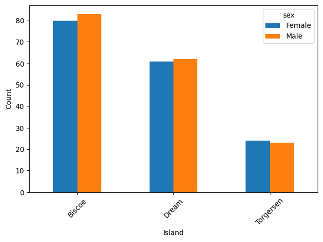
One key feature of pivot tables is that they reduce the size of the data considerably. As a result, the pivoted data usually is much easier to plot. You can create grouped bar chart from the long format:

alt.Chart(long).mark_bar().encode(
    x="island:N",
    y="count:Q",
    xOffset="sex:N",
    color="sex:N"
).properties(width=400)

This works for all pivots and their normalizations!

Saving images¶

If you would like to save the Altair plots, you need to install another library:

pip install vl-convert-python

Then add .save("myfile.png") to the plotting command (.html and .svg) work, too

Challenge¶

Examine the penguin data further:

import seaborn as sns

df = pl.from_pandas(sns.load_dataset("penguins"))
df = df.drop_nulls()

Answer the following questions:

how many penguins are in which species?
how many penguins from which species live on which island?
what is the average body mass of each species?
how long is the longest beak of each species?
what is the mean of each numerical column, per species?
what is the mean bill length and depth for each species/sex combination?

Note

The whole penguin art is inspired by the original Palmer Penguin drawings by @allison_horst